OpenStreetMap Overpass API in Python

by Michael T. Moen

OpenStreetMap (OSM): https://www.openstreetmap.org/

OSM Overpass API Documentation: https://wiki.openstreetmap.org/wiki/Overpass_API

OSM License: https://www.openstreetmap.org/copyright

The OpenStreetMap API is licensed the Open Data Commons Open Database License, which allows users to share, create, and adapt the database as long OpenStreetMap is attributed and the data is kept open.

This tutorial uses the OSMnx Python package to access the OpenStreetMap API. The examples used in this tutorial are inspired by those found in the official OSMnx Examples Gallery.

OSMnx Documentation: https://osmnx.readthedocs.io/en/stable/

OSMnx Examples Gallery: gboeing/osmnx-examples

OSMnx License: gboeing/osmnx

If you use OSMnx in your work, please cite the journal article:

Boeing, G. 2017. “OSMnx: New Methods for Acquiring, Constructing, Analyzing, and Visualizing Complex Street Networks.” Computers, Environment and Urban Systems 65, 126-139.

For more information on the usage limitations of this service, please see the Nominatim Usage Policy and the Overpass Commons documentation. Please ensure that if you use an alternative Nominatim or Overpass instance, you obey their usage policies.

These recipe examples were tested on April 1, 2024.

Import Libraries

This tutorial uses the following libraries:

import osmnx as ox
import matplotlib.pyplot as plt

1. Retrieve and Download Feature and Boundary Data

The OSMnx contains several options for retrieving GIS data associated with locations, including:

• geocode_to_gdf

• features_from_address

• features_from_bbox

• features_from_place

• features_from_point

• features_from_polygon

• features_from_xml

These methods return GeoDataFrames that can be used to work with GIS data in Python or exported and saved as other formats.

Using geocode_to_gdf to Download Boundary Data

This example uses the geocode_to_gdf method to retrieve the boundary data for the given query. This method returns a GeoDataFrame with a row for each query given. Note that the geocode_to_gdf method can also take a list of queries as an argument. In this case, the returned GeoDataFrame has a row for each query. An example of this is given later in this tutorial.

For more information on how you can use the geocode_to_gdf method, please see the OSMnx User Reference.

place = 'Alabama, USA'
alabama_gdf = ox.geocode_to_gdf(place)

# Display GeoDataFrame
alabama_gdf

	geometry	bbox_north	bbox_south	bbox_east	bbox_west	place_id	osm_type	osm_id	lat	lon	class	type	place_rank	importance	addresstype	name	display_name
0	POLYGON ((-88.47310 31.89390, -88.47264 31.875...	35.008112	30.143376	-84.888289	-88.473101	224705	relation	161950	33.258882	-86.829534	boundary	administrative	8	0.719961	state	Alabama	Alabama, United States

By default, GeoPandas saves data as an ESRI Shapefile. This can also be explicitly defined by setting the driver to ESRI Shapefile:

# Save the files to a folder called 'alabama-shapefile'
alabama_gdf.to_file('alabama-shapefile')

# This does the same thing
alabama_gdf.to_file('alabama-shapefile', driver='ESRI Shapefile')

The data can also be saved as GeoJSON by setting the driver to GeoJSON:

alabama_gdf.to_file('alabama.json', driver='GeoJSON')

We can also save the data as a GeoPackage file by setting the driver to GPKG:

alabama_gdf.to_file('alabama.gpkg', driver='GPKG')

Using features_from_address to Get Building Data

The features_from_address method takes three arguments:

• address is a string containing the address of the location of interest. This example uses the address of The University of Alabama.

• tags is a dictionary of map elements of interest in the given area. To see what elements can be queried, please see the OpenStreetMap Wiki. This example retrieves buildings of all types by using the True value for the building key.

• dist (optional) is the distance in meters from the address that is searched. By default, this value is set to 1000.

For more information on how you can use the features_from_address method, please see the OSMnx User Reference.

address = '425 Stadium Dr, Tuscaloosa, AL 35401, United States'
tags = {
    'building': True
}
gdf = ox.features_from_address(address, tags, dist=500)

# Display GeoPandas DataFrame
gdf.head()

		geometry	wheelchair	amenity	nodes	capacity	name	wikidata	wikipedia	building	parking	...	tower:type	short_name	tourism	layer	source	addr:country	name:etymology:wikidata	shelter_type	ways	type
element_type	osmid
way	120485565	POLYGON ((-87.55040 33.21352, -87.55031 33.213...	NaN	parking	[1350925632, 9262756068, 1350925631, 135092562...	NaN	North ten Hoor Parking Deck	NaN	NaN	yes	multi-storey	...	NaN	NaN	NaN	NaN	NaN	NaN	NaN	NaN	NaN	NaN
	120485567	POLYGON ((-87.55069 33.21220, -87.55059 33.212...	NaN	parking	[1350925624, 1437999814, 1350925628, 135092562...	NaN	South ten Hoor Parking Deck	NaN	NaN	yes	multi-storey	...	NaN	NaN	NaN	NaN	NaN	NaN	NaN	NaN	NaN	NaN
	120485569	POLYGON ((-87.55318 33.21223, -87.55324 33.211...	yes	NaN	[1350925625, 1350925621, 1350925622, 135092562...	NaN	Publix	NaN	NaN	yes	NaN	...	NaN	NaN	NaN	NaN	NaN	NaN	NaN	NaN	NaN	NaN
	124127809	POLYGON ((-87.55249 33.21083, -87.55246 33.211...	NaN	NaN	[1382356520, 1382356534, 1382356535, 138235657...	NaN	University Town Center B	NaN	NaN	yes	NaN	...	NaN	NaN	NaN	NaN	NaN	NaN	NaN	NaN	NaN	NaN
	124280591	POLYGON ((-87.55258 33.21171, -87.55255 33.211...	NaN	NaN	[1383629484, 1383629482, 1383629478, 138362948...	NaN	NaN	NaN	NaN	yes	NaN	...	NaN	NaN	NaN	NaN	NaN	NaN	NaN	NaN	NaN	NaN

5 rows × 47 columns

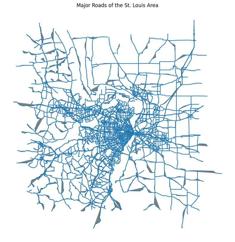
Using features_from_bbox to Get Street Features

The features_from_bbox method takes two arguments:

• bbox is tuple of floats describing the boundaries of an area of interest. This tuple must be structured as (north, south, east, west). This example looks at the area around St. Louis, MO.

• tags is a dictionary of map elements of interest in the given area. To see what elements can be queried, please see the OpenStreetMap Wiki. This example retrieves the five largest classifications of highway as defined by OpenStreetMap.

For more information on how you can use the features_from_bbox method, please see the OSMnx User Reference.

north = 39.3
south = 38.1
east = -89.6
west = -91.1
bbox = (north, south, east, west)
tags = {
    'highway': ['motorway', 'trunk', 'primary', 'secondary', 'tertiary']
}
gdf = ox.features_from_bbox(bbox=bbox, tags=tags)

Now we can graph the features above, which will be explored further in the next section.

ax = gdf.plot(fc='gray', figsize=(10, 10))
ax.axis('off')
ax.set_title('Major Roads of the St. Louis Area')
plt.show()

2. Graphing with GeoPandas

GeoPandas allows for data to be printed using the plot() function:

alabama_gdf.plot()

<Axes: >

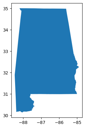
By default, GeoPandas includes latitude and longitude as the axes of the figure. This can be turned off by specifying .axis('off'). Additionally, we can suppress the output of metadata, like <Axes: > in the example above, by adding a semicolon ; to the end of the line.

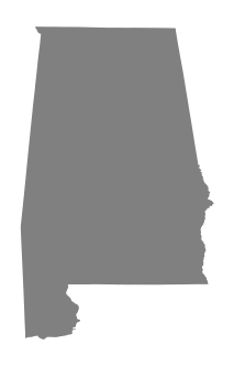
Additionally, we can modify the color of the figure with plot()’s fill color fc parameter. The figsize parameter can also be set with a tuple containing (width, height). Note that aspect ratio of image is maintained, and only the more restrictive number between width and height is used for the graph.

alabama_gdf.plot(fc='gray', figsize=(2.5, 5)).axis('off');

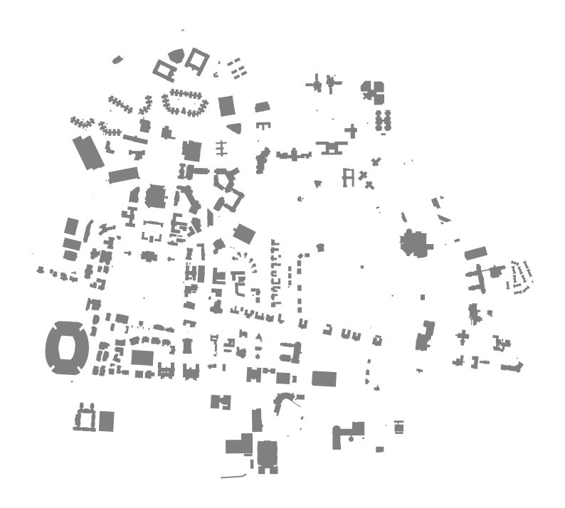
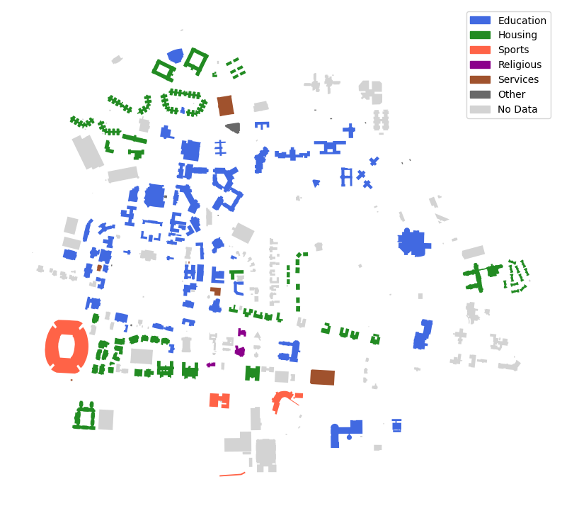
Mapping the Buildings of The University of Alabama

OpenStreetMap contains building footprint data, allowing for individual building to be plotted.

In this example, the features_from_place method is used to retrieve the data for all buildings at The University of Alabama.

place = 'University of Alabama, AL USA'
tags = {
    'building': True
}
buildings = ox.features_from_place(place, tags)
buildings.plot(fc='gray', figsize=(10, 10)).axis('off');

We can use the metadata of the buildings to color them according to their purpose. The unique tags that we must consider are given below:

buildings['building'].unique()

array(['yes', 'university', 'sports_centre', 'dormitory', 'school',
       'hotel', 'parking', 'residential', 'commercial', 'service',
       'college', 'apartments', 'house', 'shed', 'stadium', 'roof',
       'church', 'grandstand', 'yes;dormitory'], dtype=object)

Now, we can construct a dictionary assigning a color to each building type:

education_color = 'royalblue'
sports_color = 'tomato'
housing_color = 'forestgreen'
religious_color = 'darkmagenta'
services_color = 'sienna'
other_color = 'dimgray'
undefined_color = 'lightgray'

colors = {
    'university': education_color,
    'college': education_color,
    'school': education_color,

    'dormitory': housing_color,
    'hotel': housing_color,
    'residential': housing_color,
    'apartments': housing_color,
    'house': housing_color,
    'yes;dormitory': housing_color,

    'stadium': sports_color,
    'sports_centre': sports_color,
    'grandstand': sports_color,

    'church': religious_color,

    'service': services_color,
    'parking': services_color,

    'commercial': other_color,
    'roof': other_color,
    'shed': other_color,

    'yes': undefined_color,
}

Now, we can plot the buildings using the colors determined above.

import matplotlib.patches as mpatches

fig, ax = plt.subplots(figsize=(10, 10))

# Plot each building type with the appropriate color
for type in buildings['building'].unique():
    color = colors[type]
    buildings[buildings['building'] == type].plot(ax=ax, color=color)

ax.axis('off')

# Create legend
legend_handles = [
    mpatches.Patch(color=education_color, label='Education'),
    mpatches.Patch(color=housing_color, label='Housing'),
    mpatches.Patch(color=sports_color, label='Sports'),
    mpatches.Patch(color=religious_color, label='Religious'),
    mpatches.Patch(color=services_color, label='Services'),
    mpatches.Patch(color=other_color, label='Other'),
    mpatches.Patch(color=undefined_color, label='No Data'),
]
ax.legend(handles=legend_handles)

plt.show();

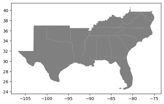
Applying a Projection on a Map

As mentioned above, the geocode_to_gdf function can take a list of places to look up as an argument. Doing so returns a single GeoDataFrame that contains the data for all of the locations. Note that each state queried is represented by a row in the GeoDataFrame.

The example below looks at the states designated as part of the South by the U.S. Census Bureau.

places = [
    'Alabama, USA', 'Mississippi, USA', 'Louisiana, USA',
    'Arkansas, USA', 'Tennessee, USA', 'Florida, USA',
    'Georgia, USA', 'South Carolina, USA', 'North Carolina, USA',
    'Kentucky, USA', 'Texas, USA', 'Oklahoma, USA',
    'Virginia, USA', 'West Virginia, USA', 'Maryland, USA',
    'District of Columbia, USA', 'Delaware, USA'
]
southern_states = ox.geocode_to_gdf(places)

# Display the top rows of the GeoPandas DataFrame
southern_states.head()

	geometry	bbox_north	bbox_south	bbox_east	bbox_west	place_id	osm_type	osm_id	lat	lon	class	type	place_rank	importance	addresstype	name	display_name
0	POLYGON ((-88.47310 31.89390, -88.47264 31.875...	35.008112	30.143376	-84.888289	-88.473101	224705	relation	161950	33.258882	-86.829534	boundary	administrative	8	0.719961	state	Alabama	Alabama, United States
1	POLYGON ((-91.65501 31.25178, -91.65491 31.250...	34.996017	30.143677	-88.097795	-91.655009	321173572	relation	161943	32.971528	-89.734850	boundary	administrative	8	0.700392	state	Mississippi	Mississippi, United States
2	POLYGON ((-94.04319 32.62108, -94.04309 32.592...	33.019594	28.854289	-88.758331	-94.043187	293608976	relation	224922	30.870388	-92.007126	boundary	administrative	8	0.713185	state	Louisiana	Louisiana, United States
3	POLYGON ((-94.61788 36.49950, -94.61772 36.498...	36.499600	33.004246	-89.644395	-94.617875	321523471	relation	161646	35.204888	-92.447911	boundary	administrative	8	0.704692	state	Arkansas	Arkansas, United States
4	POLYGON ((-90.31030 35.00429, -90.31008 35.001...	36.678118	34.982938	-81.647219	-90.310298	327458731	relation	161838	35.773008	-86.282008	boundary	administrative	8	0.720268	state	Tennessee	Tennessee, United States

southern_states.plot(fc='gray');

The project_gdf method allows us to project a GeoDataFrame to a coordinate reference system (CRS). By default, OSMnx uses UTM projection centered on your data, so please note that distance measurements may be inaccurate for areas over 620 mi (1000 km) wide. However, this can be modified by setting the to_crs tag with a string or a CRS object from pyproj.

If you would like to learn more about UTM zones, please see this article from GISGeography.com. For more information on how you can use the project_gdf method, please see the OSMnx User Reference.

projected_southern_states = ox.project_gdf(southern_states)
projected_southern_states.plot(fc='gray');

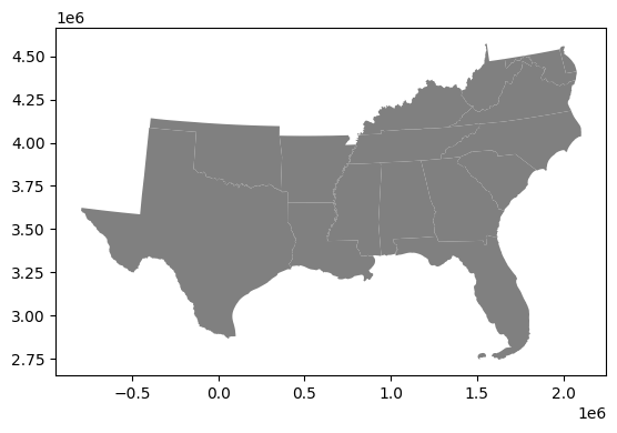
Since the projection above uses a UTM zone, the origin of the graph is where the central meridian intersects the equator. Additionally, the values on the axes are in millions of meters (or thousands of kilometers), so the distance from central Texas to central Louisiana is approximately 500 km.

3. Street Networks

The street data for a location can be retrieved with the following methods:

• graph_from_address

• graph_from_bbox

• graph_from_place

• graph_from_point

• graph_from_polygon

• graph_from_xml

The examples below all use the graph_from_place method.

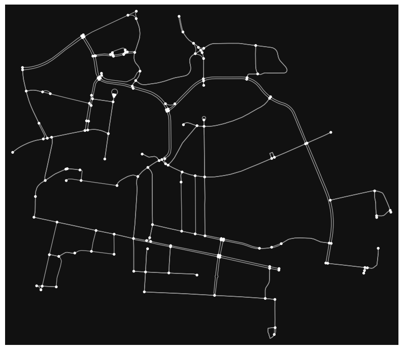
Plotting Street Networks

The graph_from_place method can be used to generate a variety of street networks by setting the network_type:

• drive

• bike

• walk

• drive_service

• all

• all_private

For more information on how you can use the graph_from_place method, please see the OSMnx User Reference.

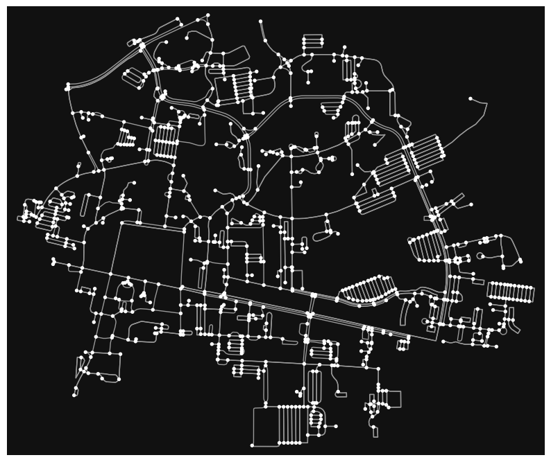
drive_graph = ox.graph_from_place('University of Alabama, Tuscaloosa, AL, USA', network_type='drive')
ox.plot_graph(drive_graph, figsize=(10, 10));

bike_graph = ox.graph_from_place('University of Alabama, Tuscaloosa, AL, USA', network_type='bike')
ox.plot_graph(bike_graph, figsize=(10, 10));

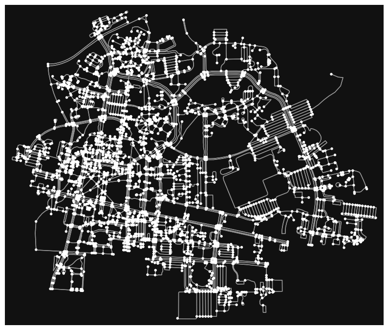
walk_graph = ox.graph_from_place('University of Alabama, Tuscaloosa, AL, USA', network_type='walk')
ox.plot_graph(walk_graph, figsize=(10, 10));

Finding the Shortest Route Between Two Nodes

Now that we have created street networks, we can use the shortest_path method to find the shortest path between two nodes.

Note that in order to use this method, the scikit-learn Python library must be installed.

origin = (33.211078599884964, -87.54927369336447)       # Coordinates of the Angelo Bruno Business Library
destination = (33.21344833663583, -87.54291076951604)   # Coordinates of the Rodgers Library

# Find the nodes nearest to each set of coordinates
origin_node = ox.distance.nearest_nodes(walk_graph, origin[1], origin[0])
destination_node = ox.distance.nearest_nodes(walk_graph, destination[1], destination[0])

# Find the shortest path and graph it
route = ox.shortest_path(walk_graph, origin_node, destination_node)
fig, ax = ox.plot_graph_route(walk_graph, route, route_color='c', node_size=0, figsize=(10, 10))

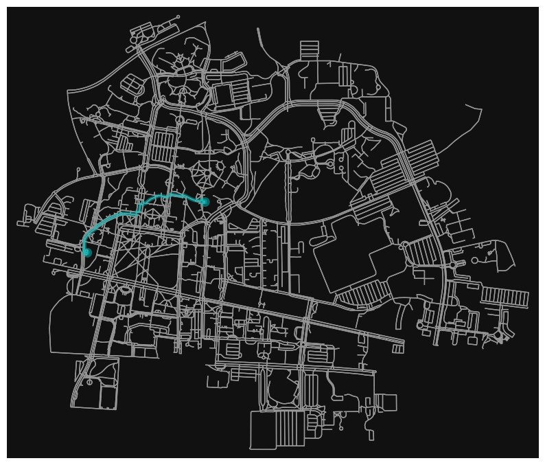
Using the route_to_gdf method, we can also find the distance of this route.

length = int(sum(ox.utils_graph.route_to_gdf(walk_graph, route, "length")["length"]))
print(f'The route is {length} meters.')

The route is 850 meters.