World Bank API in Python#
by Avery Fernandez
See the World Bank API documentation
These recipe examples were tested on February 13, 2022
1. Get list of country iso2Codes and names#
First, import libraries needed to pull data from the API:
from time import sleep
import requests
from pprint import pprint
For obtaining data from the World Bank API, it is helpful to first obtain a list of country codes and names.
# define root WorldBank API
api = 'https://api.worldbank.org/v2/'

# define api url for getting country code data
country_url = api + 'country/?format=json&per_page=500'

# read the url and import data as JSON data
country_data = requests.get(country_url).json()[1]
pprint(country_data[0]) # shows first bit of data
print(len(country_data)) # shows the size of data
{'adminregion': {'id': '', 'iso2code': '', 'value': ''},
 'capitalCity': 'Oranjestad',
 'id': 'ABW',
 'incomeLevel': {'id': 'HIC', 'iso2code': 'XD', 'value': 'High income'},
 'iso2Code': 'AW',
 'latitude': '12.5167',
 'lendingType': {'id': 'LNX', 'iso2code': 'XX', 'value': 'Not classified'},
 'longitude': '-70.0167',
 'name': 'Aruba',
 'region': {'id': 'LCN',
            'iso2code': 'ZJ',
            'value': 'Latin America & Caribbean '}}
299
# Extract out iso2code from countries data
country_iso2Code = []
for isos in range(len(country_data)):
    country_iso2Code.append(country_data[isos]["iso2Code"])
pprint(country_iso2Code[0:10]) # shows first 10
print(len(country_iso2Code)) # shows the size of data
['AW', 'ZH', 'AF', 'A9', 'ZI', 'AO', 'AL', 'AD', '1A', 'AE']
299
# Extract out country names
country_name = []
for names in range(len(country_data)):
    country_name.append(country_data[names]["name"])
pprint(country_name[0:10]) # shows first 10
print(len(country_name)) # shows the size of data
['Aruba',
 'Africa Eastern and Southern',
 'Afghanistan',
 'Africa',
 'Africa Western and Central',
 'Angola',
 'Albania',
 'Andorra',
 'Arab World',
 'United Arab Emirates']
299
# now combine country_iso2Code and country name
country_iso2code_name = {country_iso2Code[i]: country_name[i] for i in range(len(country_iso2Code))}
print(len(country_iso2code_name)) # shows the size of data
299
Now we know the country iso2Codes which we can use to pull specific indicator data for countries.
2. Compile a Custom Indicator Dataset#
There are many availabe indicators: https://data.worldbank.org/indicator
We wll select three indicators for this example:
Scientific and Technical Journal Article Data = IP.JRN.ARTC.SC
Patent Applications, residents = IP.PAT.RESD
GDP per capita (current US$) Code = NY.GDP.PCAP.CD
Note that these three selected indictaors have a CC-BY 4.0 license We will compile this indicator data for the United States (US) and United Kingdom (GB)
indicators = ['IP.JRN.ARTC.SC','IP.PAT.RESD','NY.GDP.PCAP.CD']
Generate the web API urls we need for U.S and retrieve the data.
US_api_URL = {}
US_indicator_data = {}
for number in range(len(indicators)):
    US_api_URL = api + 'country/US/indicator/' + indicators[number] + '/?format=json&per_page=500'
    US_indicator_data[number] = requests.get(US_api_URL).json()
    sleep(1)
Generate web API urls we need for the UK (GB)
UK_api_URL = {}
UK_indicator_data = {}
for number in range(len(indicators)):
    UK_api_URL = api + 'country/GB/indicator/' + indicators[number] + '/?format=json&per_page=500'
    UK_indicator_data[number] = requests.get(UK_api_URL).json()
    sleep(1)
Now we need to extract the data and compile for analysis.
column 1: year
column 2: Scientific and Technical Journal Article Data = IP.JRN.ARTC.SC
column 3: Patent Applications, residents = IP.PAT.RESD
column 4: GDP per capita (current US$) Code = NY.GDP.PCAP.CD
NOTE: float(x or ‘nan’) is used to get rid of empty cells.
# US Data compilation
US_data = {}
for years in range(len(US_indicator_data[0][1])):
    US_data[int(US_indicator_data[0][1][years]["date"])] = [float(US_indicator_data[0][1][years]["value"] or 'nan'),
                                                            float(US_indicator_data[1][1][years]["value"] or 'nan'),
                                                            float(US_indicator_data[2][1][years]["value"] or 'nan')]
pprint(US_data)
{1960: [nan, nan, 3007.12344537862],
 1961: [nan, nan, 3066.56286916615],
 1962: [nan, nan, 3243.84307754988],
 1963: [nan, nan, 3374.51517105082],
 1964: [nan, nan, 3573.94118474743],
 1965: [nan, nan, 3827.52710972039],
 1966: [nan, nan, 4146.31664631665],
 1967: [nan, nan, 4336.42658722171],
 1968: [nan, nan, 4695.92339043178],
 1969: [nan, nan, 5032.14474262003],
 1970: [nan, nan, 5234.2966662115],
 1971: [nan, nan, 5609.38259952519],
 1972: [nan, nan, 6094.01798986165],
 1973: [nan, nan, 6726.35895596695],
 1974: [nan, nan, 7225.69135952566],
 1975: [nan, nan, 7801.45666356443],
 1976: [nan, nan, 8592.25353727612],
 1977: [nan, nan, 9452.57651914511],
 1978: [nan, nan, 10564.9482220275],
 1979: [nan, nan, 11674.1818666548],
 1980: [nan, 62098.0, 12574.7915062163],
 1981: [nan, 62404.0, 13976.10539252],
 1982: [nan, 63316.0, 14433.787727053],
 1983: [nan, 59391.0, 15543.8937174925],
 1984: [nan, 61841.0, 17121.2254849995],
 1985: [nan, 63673.0, 18236.8277265009],
 1986: [nan, 65195.0, 19071.2271949295],
 1987: [nan, 68315.0, 20038.9410992658],
 1988: [nan, 75192.0, 21417.0119305191],
 1989: [nan, 82370.0, 22857.1544330056],
 1990: [nan, 90643.0, 23888.6000088133],
 1991: [nan, 87955.0, 24342.2589048189],
 1992: [nan, 92425.0, 25418.9907763319],
 1993: [nan, 99955.0, 26387.2937338171],
 1994: [nan, 107233.0, 27694.853416234],
 1995: [nan, 123962.0, 28690.8757013347],
 1996: [nan, 106892.0, 29967.7127181749],
 1997: [nan, 119214.0, 31459.1389804773],
 1998: [nan, 134733.0, 32853.6769523009],
 1999: [nan, 149251.0, 34513.5615037271],
 2000: [304781.56, 164795.0, 36334.9087770589],
 2001: [305612.91, 177513.0, 37133.2428088526],
 2002: [319307.62, 184245.0, 38023.1611144021],
 2003: [329398.86, 188941.0, 39496.4858751381],
 2004: [353853.49, 189536.0, 41712.8010675545],
 2005: [384572.94, 207867.0, 44114.7477810544],
 2006: [385515.0, 221784.0, 46298.7314440927],
 2007: [391909.59, 241347.0, 47975.9676958038],
 2008: [393978.95, 231588.0, 48382.5584490552],
 2009: [399350.31, 224912.0, 47099.9804711343],
 2010: [408817.1, 241977.0, 48466.6576026922],
 2011: [423958.81, 247750.0, 49882.5581321495],
 2012: [427996.8, 268782.0, 51602.9310457907],
 2013: [429570.05, 287831.0, 53106.5367672165],
 2014: [433192.28, 285096.0, 55049.9883272312],
 2015: [429988.89, 288335.0, 56863.3714957652],
 2016: [427264.63, 295327.0, 58021.4004997125],
 2017: [432216.49, 293904.0, 60109.6557260477],
 2018: [422807.71, 285095.0, 63064.4184096731],
 2019: [nan, 285113.0, 65279.5290260953],
 2020: [nan, nan, 63413.5138584508]}
UK Data extraction
column 1: year
column 2: Scientific and Technical Journal Article Data = IP.JRN.ARTC.SC
column 3: Patent Applications, residents = IP.PAT.RESD
column 4: GDP per capita (current US$) Code = NY.GDP.PCAP.CD
NOTE: float(x or ‘nan’) is used to get rid of empty cells.
UK_data = {}
for years in range(len(UK_indicator_data[0][1])):
    UK_data[int(UK_indicator_data[0][1][years]["date"])] = [float(UK_indicator_data[0][1][years]["value"] or 'nan'),
                                                            float(UK_indicator_data[1][1][years]["value"] or 'nan'),
                                                            float(UK_indicator_data[2][1][years]["value"] or 'nan')]
pprint(UK_data)
{1960: [nan, nan, 1397.5948032844],
 1961: [nan, nan, 1472.38571407868],
 1962: [nan, nan, 1525.77585271032],
 1963: [nan, nan, 1613.45688373392],
 1964: [nan, nan, 1748.2881176141],
 1965: [nan, nan, 1873.56777435421],
 1966: [nan, nan, 1986.74715869685],
 1967: [nan, nan, 2058.78188198056],
 1968: [nan, nan, 1951.75859587532],
 1969: [nan, nan, 2100.66786858672],
 1970: [nan, nan, 2347.54431773747],
 1971: [nan, nan, 2649.80151387223],
 1972: [nan, nan, 3030.43251411977],
 1973: [nan, nan, 3426.27622050378],
 1974: [nan, nan, 3665.8627976419],
 1975: [nan, nan, 4299.74561799284],
 1976: [nan, nan, 4138.16778761535],
 1977: [nan, nan, 4681.43993173038],
 1978: [nan, nan, 5976.93816899991],
 1979: [nan, nan, 7804.76208051155],
 1980: [nan, 19612.0, 10032.062080015],
 1981: [nan, 20808.0, 9599.30622221965],
 1982: [nan, 20530.0, 9146.07735701852],
 1983: [nan, 19893.0, 8691.51881306514],
 1984: [nan, 19093.0, 8179.19444064991],
 1985: [nan, 19672.0, 8652.21654247593],
 1986: [nan, 20040.0, 10611.112210096],
 1987: [nan, 19945.0, 13118.586534629],
 1988: [nan, 20536.0, 15987.1680775688],
 1989: [nan, 19732.0, 16239.2821960944],
 1990: [nan, 19310.0, 19095.4669984608],
 1991: [nan, 19230.0, 19900.7266505069],
 1992: [nan, 18848.0, 20487.1707852878],
 1993: [nan, 18727.0, 18389.0195675099],
 1994: [nan, 18384.0, 19709.2380983653],
 1995: [nan, 18630.0, 23206.5685593776],
 1996: [nan, 18184.0, 24438.531169209],
 1997: [nan, 17938.0, 26742.9848472166],
 1998: [nan, 19530.0, 28269.322509823],
 1999: [nan, 21333.0, 28726.8572106345],
 2000: [77244.9, 22050.0, 28223.0675706515],
 2001: [73779.92, 21423.0, 27806.4488245133],
 2002: [74814.46, 20624.0, 30049.8963232066],
 2003: [75564.08, 20426.0, 34487.4675722539],
 2004: [79249.97, 19178.0, 40371.7108259838],
 2005: [84940.1, 17833.0, 42132.0907219815],
 2006: [88142.47, 17484.0, 44654.0969208924],
 2007: [91212.76, 17375.0, 50653.2569148306],
 2008: [91357.74, 16523.0, 47549.3486286006],
 2009: [93803.37, 15985.0, 38952.2110262455],
 2010: [93791.51, 15490.0, 39688.6149684498],
 2011: [95820.1, 15343.0, 42284.8844902996],
 2012: [98144.92, 15370.0, 42686.8000524926],
 2013: [99228.41, 14972.0, 43713.8141242308],
 2014: [99384.79, 15196.0, 47787.2412984884],
 2015: [99616.02, 14867.0, 45404.5677734722],
 2016: [99366.17, 13876.0, 41499.5557033073],
 2017: [99128.72, 13301.0, 40857.7555829627],
 2018: [97680.9, 12865.0, 43646.9519711493],
 2019: [nan, 12061.0, 43070.4983595888],
 2020: [nan, nan, 41124.5347686731]}
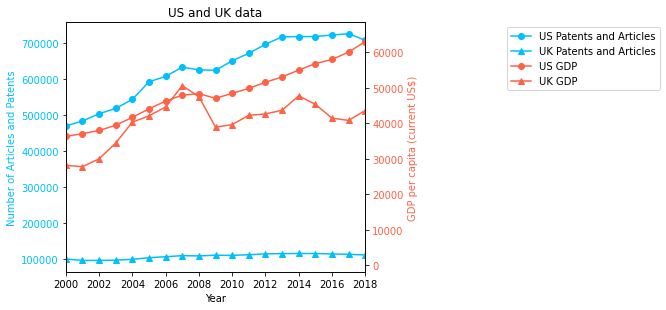
3. Plot Indicator data#
Create a line plot of US/UK Number of Scientific and Technical Journal Articles and Patents by year
import matplotlib.pyplot as plt
from matplotlib.pyplot import figure

# US Data
US_patentsandarticles = []
US_gdp = []
data_years = list(US_data.keys())
data_years.sort()
for years in data_years:
    US_patentsandarticles.append(US_data.get(years)[0]+US_data.get(years)[1])
    US_gdp.append(US_data.get(years)[2])

# UK Data
UK_patentsandarticles = []
UK_gdp = []
data_years = list(UK_data.keys())
data_years.sort()
for years in data_years:
    UK_patentsandarticles.append(UK_data.get(years)[0]+UK_data.get(years)[1])
    UK_gdp.append(UK_data.get(years)[2])

fig, ax1 = plt.subplots()
ax1.set_ylabel("Number of Articles and Patents", {'color': 'deepskyblue'})
ax1.plot(data_years,US_patentsandarticles, label = "US Patents and Articles",
         marker="o", color="deepskyblue")
ax1.plot(data_years,UK_patentsandarticles, label = "UK Patents and Articles",
         marker="^", color="deepskyblue")
ax1.tick_params(axis='y', labelcolor="deepskyblue")

ax2 = ax1.twinx()
ax2.set_ylabel("GDP per capita (current US$)", {'color': 'tomato'})
ax2.plot(data_years,US_gdp, label = "US GDP", marker="o", color="tomato")
ax2.plot(data_years,UK_gdp, label = "UK GDP", marker="^", color="tomato")
ax2.tick_params(axis='y', labelcolor="tomato")

fig.tight_layout()
ax1.set_xlabel("Year")
plt.title("US and UK data")
plt.xlim(2000,2018)

lines_labels = [ax.get_legend_handles_labels() for ax in fig.axes]
lines, labels = [sum(lol, []) for lol in zip(*lines_labels)]
plt.legend(lines, labels, bbox_to_anchor=(2, 1), ncol=1)
#fig.legend(lines, labels,loc = 'upper right')
plt.show()